はじめに

　本記事をご覧いただきありがとうございます。ドコモアドベントカレンダー8日目の記事になります。初めまして。NTTドコモR&D戦略部新入社員の武田です。業務では主に弊社の先進技術を活用したメタコミュニケーションサービス「MetaMe®」（メタミー）の技術実装を担当しています。

私は学生時代、人々の動きや行動パターンを実データから分析し、災害時の安心・安全な避難を実現するためのシミュレーションや最適化に関する研究に従事しておりました。現在仮想空間内においても「ユーザの流れ」や「ユーザの行動」に注目し、技術実装を行っています。群衆の動きに関するサーベイを進める中で、「同期現象」に関する論文を目にし、その仕組みに強く興味を持ちました。

そこで本記事では、「同期現象」を数理モデルで表現した2種類のモデルをとりあげ、Pythonを用いた実装を通して、その仕組みをより深く理解することに挑戦します。

対象者

生態系や社会的な相互作用を数理モデルで表現することに興味がある方
Pythonでの実装を通じて同期モデルを学びたい方

内容

同期現象とは？
同期現象の数理モデル
- 「蔵本モデル」の概要と実装
- 「モバイル振動子ネットワークの同期モデル」の概要と実装
まとめ

実行環境

OS：Windows 11 Pro
エディタ：Visual Studio Code 1.95.2
Python：3.9.1

同期現象とは

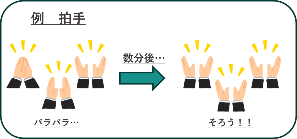
　世の中には「自然に揃ってしまう」現象が数多く存在します。例えばイベント会場での観客の拍手。最初はバラバラだった拍手が、気がつくと会場全体で揃っている——そんな経験をしたことがある方も多いのではないでしょうか？他にも、初夏の夜にホタルが一斉に点滅する様子や、心臓の細胞がリズムを合わせて拍動する動き、メトロノームが同じタイミングで揺れ始めることも「自然に揃ってしまう」現象の一例です。このように周囲の影響を受けながら、徐々に足並みが揃う現象を「同期現象」といいます。

同期現象の数理モデル

　では、この「同期現象」は単なる偶然の一致により生まれるのでしょうか？実は、この現象には数学的な理論が関わっています。複数の個体が互いに影響し合いながら、徐々に足並みを揃える現象は、数理モデルを用いて説明することができます。本記事では同期現象を記述する2種類の数理モデルを、概要、数式、実装に分けてご紹介します。

「蔵本モデル」について

概要

「蔵本モデル」は同期現象を説明する代表的な数理モデルです *1。このモデルは、日本の物理学者である蔵本由紀教授により提案されました。振動する個体（振動子）が互いに影響を与え合いながらリズムを揃えていく過程を数学的に記述しています。

数式

$\displaystyle{ \frac{d\theta_i}{dt}=ω_i + \frac{K}{N}\sum_{j=1}^{N} \sin(\theta_j-\theta_i) 　{i}=1 , ···{,N} }$

　パラメータ

$\omega_i$ ：固有振動数
振動子 $i$ が固有に保持する位相の変化する大きさ度合い
${\sin(\theta_j - \theta_i)}$ ：位相差
振動子 $j$ が振動子 $i$ に与える影響の大きさ
$K$ ：結合強度
振動子同士の影響度合い
$N$ ：振動子の数
平均化

このモデルは「自分自身のリズム (第1項)」と「周辺のリズムの影響 (第2項)」を合わせながら、最終的に他の振動子と足並みを揃えていく過程を示しています。ここで重要となるのはパラメータ $K$ (結合強度)です。前述の通り、 ${\sum_{j=1}^{N} \sin(\theta_j-\theta_i)}$ は相互作用項であり、 $K$ は相互作用項の大きさを決めるパラメータになります。 $K$ の値が大きいほど、他の振動子から受ける影響が大きくなるため、同期現象が起こりやすくなります。

実装

ここでは蔵本モデルの実装を行います。著者の実行環境は冒頭で示した通りです。今回は結合強度 $K$ の値を変化させることで、同期の度合いにどのような変化が生じるのかを確認します。出力として、タイムステップごとの各振動子の位相状態を示すグラフと、その様子を可視化したアニメーションを作成します。

「蔵本モデル」サンプルコード　

import numpy as np
import os
import matplotlib.cm as cm
import matplotlib.pyplot as plt
import scipy.spatial.distance as distance
from tqdm import tqdm
import matplotlib.animation as animation
from mpl_toolkits.axes_grid1 import make_axes_locatable

"""Update oscillator phase (Kuramoto model)"""
def update_phases(phases):
   phase_mat = np.tile(phases, N).reshape(N, N)
   coupling = (K / N) * np.sum(np.sin(phase_mat - phase_mat.T), axis=1)
   new_phases = phases + coupling
   return np.mod(new_phases, 2 * np.pi)  

"""Generate positions randomly"""
def make_positions_random():
   pos_x_t = np.random.uniform(0, L, N)
   pos_y_t = np.random.uniform(0, L, N)
   return pos_x_t, pos_y_t

"""Generate animation"""
def plot_animation(timerange, pos_x, pos_y, phase):
   fig_scale = 0.1
   fig = plt.figure(figsize=(L*fig_scale, L*fig_scale), dpi=100.0)
   ax1 = plt.subplot2grid((1, 1), (0, 0))
   ax1.axis('square')
   ax1.set_xlim(0, L); ax1.set_ylim(0, L)
   ax1.tick_params(labelbottom=False, bottom=False,
                     labelleft=False, left=False,
                     labelright=False, right=False,
                     labeltop=False, top=False)
   # Create animation   
   all_ims, traj_x, traj_y = [],  [pos_x], [pos_y]
   for s in range(timerange):
         ims = []
         im = ax1.scatter(pos_x, pos_y, s=60, c=phase[s], cmap=cm.seismic,
                        vmin=0, vmax=2 * np.pi,
                        linewidths=0.5, edgecolors='grey')   
         if s == 0:
            divider = make_axes_locatable(ax1) 
            cax = divider.append_axes('right', size='5%', pad=0.1) 
            fig.colorbar(im, cax=cax)  
         # Show step
         im_text = ax1.text(L/2 - 8, L + 0.5, f'Step={s}', size=20)
         ims += [im, im_text]
         # Plot
         if s != 0:
            traj_x.append(pos_x)
            traj_y.append(pos_y)
            ims.extend(ax1.plot(traj_x[-2:], traj_y[-2:], c="k", alpha=0.3))
         all_ims.append((ims))

   ani = animation.ArtistAnimation(fig, all_ims, interval=50, repeat=True)
   plt.show()
   ani.save(f'{folderpath}/Movie.mp4', writer="ffmpeg", fps=10)

if __name__ == "__main__":
   # Parameters
   K, delta, N, T, L = 0.1, 0.5, 100, 1000, 100
   
   # Fix seed
   np.random.seed(3)
   # Generate initial positions and phases
   phase_t = np.zeros((T, N))
   phase_t[0] = np.random.uniform(0, 2 * np.pi, N)
   pos_x_t, pos_y_t = make_positions_random(N, L)
   
   phase_diffs, sync_step = [], -1
   folderpath = './SaveKuramoto'
   os.makedirs(f'{folderpath}', exist_ok=True)

   # Start simulation
   for t in tqdm(range(1, T)):
         # Update phases
         phase = update_phases(phase_t[t-1])
         phase_t[t] = phase
         # Calculate evaluation function
         avg_phase_diff = np.sqrt(np.sum([(phase[i] - phase[j]) ** 2 for i in range(N) for j in range(i+1, N)]) * 2 / (N * (N-1)))
         phase_diffs.append(avg_phase_diff)
         if avg_phase_diff < delta and sync_step == -1:
            sync_step = t 
   print(f'Synchronization achieved at timestep {sync_step}')
   

   # Plot position information
   plt.figure(figsize=(6, 6))
   plt.title(f'Position')
   plt.scatter(pos_x_t, pos_y_t)
   plt.axis('Square')
   plt.xlim([0, L]), plt.ylim([0, L])
   plt.grid()
   plt.savefig(f'{folderpath}/Position.png')
   plt.show()

   # Plot the phase state of each oscillator
   plt.title(f'Phase')
   plt.plot(phase_t)
   plt.savefig(f'{folderpath}/Phase.png')
   plt.show()

   # Plot error rate
   plt.title(f'Error')
   plt.plot(phase_diffs)
   plt.ylim([0, 5])
   plt.savefig(f'{folderpath}/Error.png')
   plt.show()

   # Animation generation
   plot_animation(400, pos_x_t, pos_y_t, phase_t)

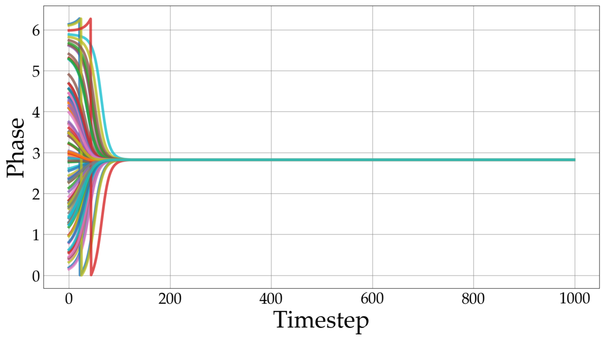
実装結果

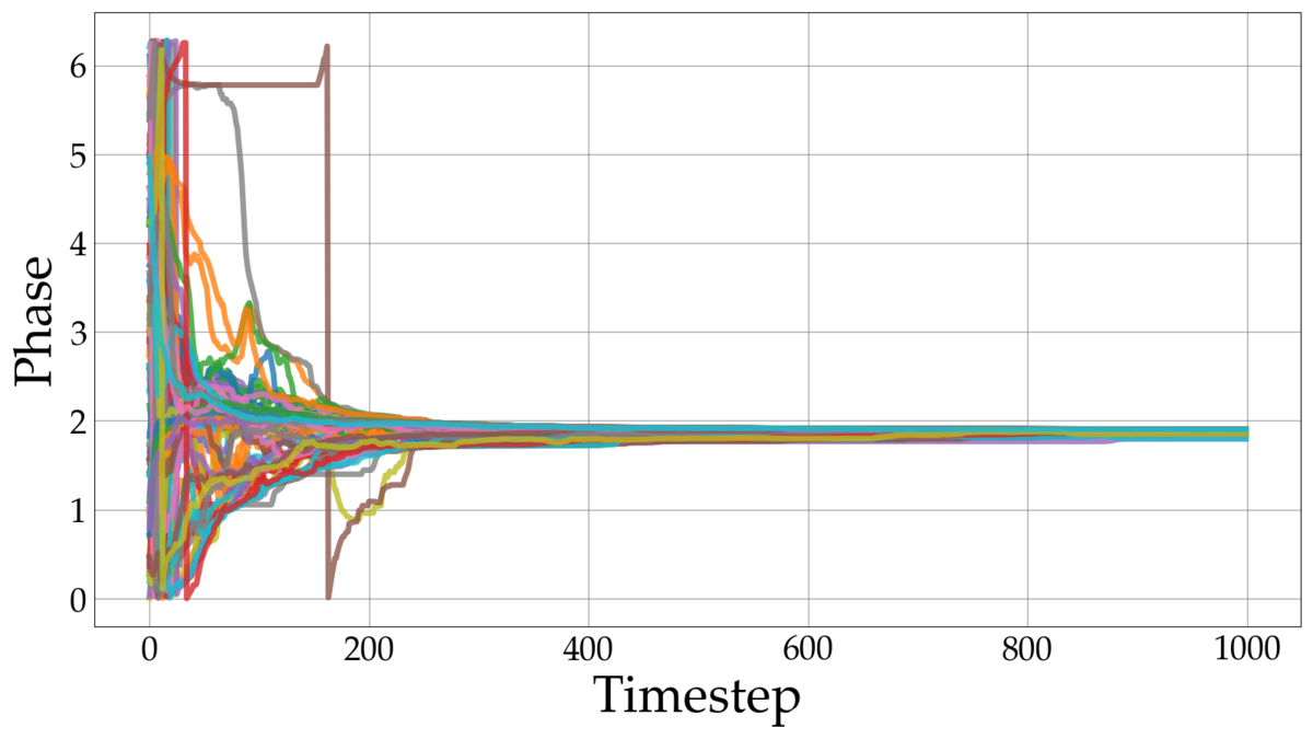
$K=0.1$ の時
空間内の振動子が初期のタイムステップで同期することを確認できます。

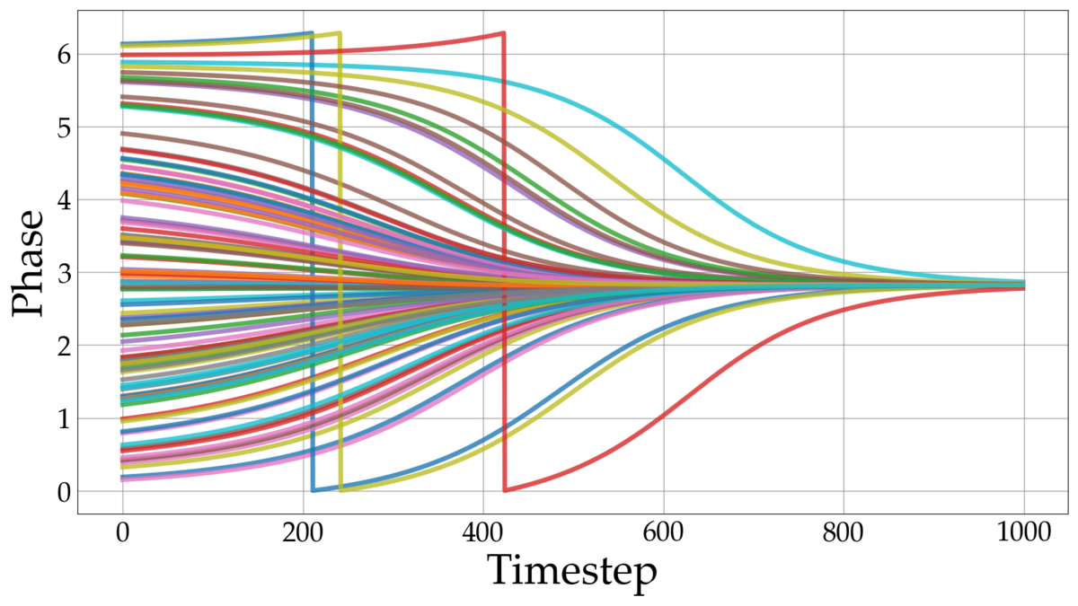
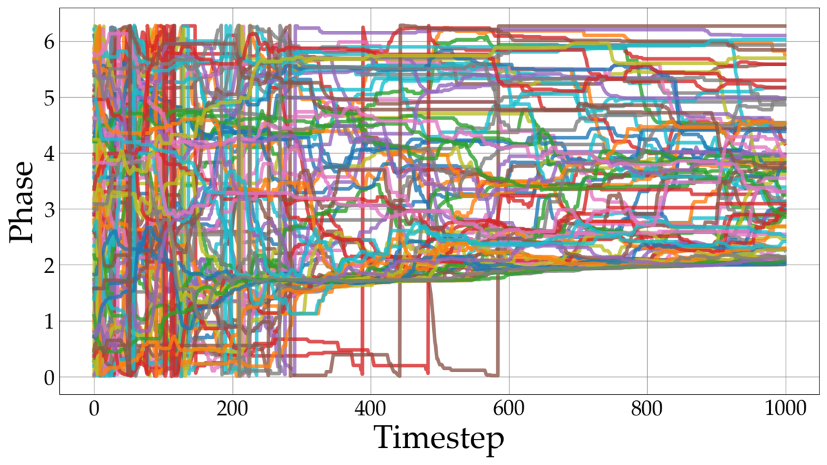
$K=0.01$ の時
$K=0.1$ と比較すると、全体が同期するタイムステップが遅いことがわかります。また、アニメーションでは、 $400$ ステップ時点で全体の同期が達成されていない様子が確認できます。

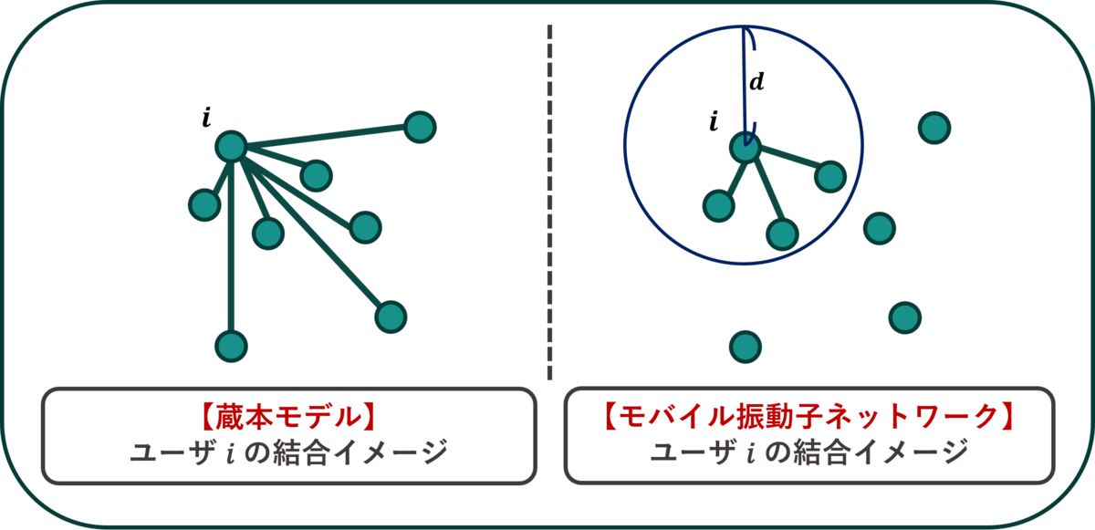
　これまでに紹介した蔵本モデルは、振動子が固定位置にあり、相互作用が瞬時に行われる静的なネットワークを前提としています。しかし「イベント会場での拍手の同期」や「蛍の点滅の同期」などの現象を考えると、人々や蛍が自由に動き回る状況も想定する必要があります。このような理由から、空間変動を考慮し、局所的な同期の形成が可能な蔵本モデルの拡張が提案されています。本記事ではこの拡張モデルとして「モバイル振動子ネットワークの同期モデル」を紹介します。

「モバイル振動子ネットワークの同期モデル」について

概要

「モバイル振動子ネットワークの同期モデル」は、移動可能な振動子が、互いに影響を与え合いながらリズムを揃える現象を表すモデルです *2。このネットワークでは、振動子が空間内を自由に移動し、近接する振動子のみと影響を与え合いながら、徐々に全体が同じリズムに揃う過程を記述しています。

数式

$\displaystyle{ φ_i(t+1)=φ_i(t)+σ\sum_{j, d_{ij}\lt d}\sin[φ_j(t)−φ_i(t)] }$

パラメータ

$\varphi_i(t)$ ：振動子 $i$ の内部状態
振動子 $i$ が固有に持っている位相の変化する大きさ度合い
${\sin[\varphi_j(t)−\varphi_i(t)]}$ ：位相差
振動子 $j$ が振動子 $i$ に与える影響の大きさ
$\sigma$ ：結合強度
振動子同士の影響度合い
$d$ ：距離の閾値
振動子同士が相互作用するための距離の基準値

　モバイル振動子ネットワークの同期モデルと蔵本モデルは振動子のリズムを揃える「同期のメカニズム」は共通しています。しかし、両者には大きな違いがあります。それは振動子間の相互作用が距離に依存するかどうかです。モバイル振動子ネットワークでは、振動子 $i$ と $j$ の距離 $d_{ij}$ が基準値 $d$ 未満である場合のみ、互いに影響を与え合います。このように距離に基づく相互作用の仕組みにより、振動子の位置や移動による空間の変化が同期に反映され、局所的な同期の形成も可能になります。

実装

　ここではモバイル振動子ネットワークの同期モデルの実装を行います。振動子の移動方向は論文 *3を参考にしました。今回は相互作用が働く距離の基準値 $d$ の値を変化させることで、同期の度合いにどのような変化が生じるのかを確認します。出力は蔵本モデルの実装時と同様にタイムステップごとの各振動子の位相状態を示すグラフとその様子を可視化したアニメーションを作成します。

「モバイル振動子ネットワークの同期モデル」サンプルコード　

import numpy as np
import os
import matplotlib.cm as cm
import matplotlib.pyplot as plt
import scipy.spatial.distance as distance
from tqdm import tqdm
import matplotlib.animation as animation
from mpl_toolkits.axes_grid1 import make_axes_locatable

"""Update oscillator phase (mobile oscillator network)"""
def update_phases(positions, phases):
   position_mat = positions
   dist = distance.pdist(position_mat)
   dist_mat = distance.squareform(dist)
   couple_df = (dist_mat <= interaction_range).astype(int)
   couple_df[range(N), range(N)] = 0
   phase_mat = np.tile(phases, N).reshape(N,N)
   coupling = sigma * np.sum(np.sin((phase_mat - phase_mat.T) * couple_df), axis=1)
   new_phases = phases + coupling
   return  np.mod(new_phases, 2 * np.pi)

"""Generate a variable to store position information 
   (+ randomly generate initial positions)"""
def make_positions_random():
   pos_x_t = np.zeros((T, N))
   pos_y_t = np.zeros((T, N))
   pos_x_t[0] = np.random.uniform(0, L, N)
   pos_y_t[0] = np.random.uniform(0, L, N)
   return pos_x_t, pos_y_t

"""Generate a variable to store phases and phase angles 
   (+ randomly generate initial phases and phase angles)"""
def make_anglesphases():
   phase_t = np.zeros((T, N))
   xi_t = np.zeros((T, N))
   phase_t[0] = np.random.uniform(0, 2*np.pi, N)   
   xi_t[0] = np.random.uniform(0, 2*np.pi, N)
   return  phase_t, xi_t 

"""Generate animation"""
def plot_animation(timerange, pos_x, pos_y, phase):
   fig_scale = 0.1
   fig = plt.figure(figsize=(L * fig_scale, L * fig_scale), dpi=100.0)
   ax1 = plt.subplot2grid((1, 1), (0, 0))
   ax1.axis('square')
   ax1.set_xlim(0, L); ax1.set_ylim(0, L)
   ax1.tick_params(labelbottom=False, bottom=False,
                  labelleft=False, left=False,
                  labelright=False, right=False,
                  labeltop=False, top=False)
   # Create animation  
   all_ims, traj_x, traj_y = [], [pos_x[0]], [pos_y[0]]
   for s in range(timerange):
      ims = []
      im = ax1.scatter(pos_x[s],  pos_y[s], s=60, c=phase[s], cmap=cm.seismic,
                        vmin=0, vmax=2 * np.pi,
                        linewidths=0.5, edgecolors='grey')
      if s == 0:
         divider = make_axes_locatable(ax1) 
         cax = divider.append_axes('right', size='5%', pad=0.1) 
         fig.colorbar(im, cax=cax)
      # Show step
      im_text = ax1.text(L/2 - 8, L + 0.5 , f'Step={s}', size=20)
      ims = ims + [im, im_text]
      # Show the coupling range
      # im_circle = ax1.scatter(pos_x[s], pos_y[s], s = interaction_range ** 2, alpha = 0.005, color = 'grey', zorder = 10000)
      # Plot
      if s != 0 and np.mod(s,tau_m) == 0:
         traj_x.append(pos_x[s])
         traj_y.append(pos_y[s])
         ims.extend((ax1.plot(traj_x[-2:], traj_y[-2:], c="k", alpha=0.3)))
      all_ims.append((ims))

   ani = animation.ArtistAnimation(fig, all_ims, interval=50, repeat=True)
   plt.show()
   ani.save(f'{folderpath}/Movie.mp4', writer="ffmpeg", fps=10)

if __name__ == "__main__":
   # Parameters
   sigma, delta, N, T, L = 0.08, 0.5, 100, 1000, 100
   # NewParameters
   interaction_range = 5.0        # Interaction range
   v = 2                           # Speed
   tau_m = 1

   # Fix seed
   np.random.seed(3)
   # Generate initial positions, angles and phases
   pos_x_t, pos_y_t = make_positions_random()
   phase_t, xi_t = make_anglesphases()

   phase_diffs, sync_step = [], -1
   folderpath = './SaveMobile'
   os.makedirs(f'{folderpath}', exist_ok=True)

   # Start simulation
   for t in tqdm(range(1, T)):
      if np.mod(t, tau_m)==0:
         # Generate phase angles
         xi_t[t] = np.random.uniform(0, 2 * np.pi, N)
         pos_x_t[t] = np.minimum(pos_x_t[t-1] + v * np.cos(xi_t[t]), np.ones(N) * L )
         pos_y_t[t] = np.minimum(pos_y_t[t-1] + v * np.sin(xi_t[t]), np.ones(N) * L )
      else:
         # Inherit information from the previous timestep
         xi_t[t] = xi_t[t-1]
         pos_x_t[t] = pos_x_t[t-1]
         pos_y_t[t] = pos_y_t[t-1]
      # Update phases
      phase = update_phases(np.vstack([pos_x_t[t], pos_y_t[t]]).reshape(N, 2), phase_t[t-1])
      phase_t[t] = phase
      # Calculate evaluation function
      avg_phase_diff = np.sqrt(np.sum([(phase[i] - phase[j]) ** 2 for i in range(N) for j in range(i+1, N)]) * 2 / (N * (N-1)))
      phase_diffs.append(avg_phase_diff)
      if avg_phase_diff < delta and sync_step == -1:
         sync_step = t
   print(f'Synchronization achieved at timestep {sync_step}')
   

   # Plot position information
   plt.figure(figsize=(6, 6))
   plt.title(f'Position')
   plt.scatter(pos_x_t[:, :], pos_y_t[:, :])
   plt.axis('Square')
   plt.xlim([0, L]), plt.ylim([0, L])
   plt.grid()
   plt.savefig(f'{folderpath}/Position.png')
   plt.show()

   # Plot the phase state of each oscillator
   plt.title(f'Phase')
   plt.plot(phase_t)
   plt.savefig(f'{folderpath}/Phase.png')
   plt.show()

   # Plot error rate
   plt.title(f'Error')
   plt.plot(phase_diffs)
   plt.ylim([0, 5])
   plt.savefig(f'{folderpath}/Error.png')
   plt.show()

   # Generate animation 
   plot_animation(400, pos_x_t, pos_y_t, phase_t)

実装結果

$d=5$ の時
近接する振動子同士の同期は見られるものの、空間全体での同期は達成されていません。

$d=15$ の時
初期ステップでは近接する振動子同士の同期が始まり、その後徐々に空間全体が同期していく様子が確認できます。

まとめ

　本記事では、同期現象を説明する2種類の数理モデルについて、概要、数式、実装という観点からご紹介いたしました。今回の内容が読者の皆様にとって同期現象への理解を深める一助となれば幸いです。今後は、これらのモデルを仮想空間上で再現し、そこから新しいインタラクティブな体験を創出することを目指しています。興味を持たれた方は、ぜひ実際にコードを動かして、同期現象の魅力を実感してみてください！

*1:Y. Kuramoto, Self-entrainment of a population of coupled non-linear oscillators, International Symposium on Mathematical Problems in Theoretical Physics, pp. 420–422. Lecture Notes in Phys., 39. Springer, Berlin, 1975.

*2:N. Fujiwara, J. Kurths, A. Díaz-Guilera, "Synchronization in networks of mobile oscillators," Physical Review E—Statistical, Nonlinear, and Soft Matter Physics, Vol. 83, No. 2, p. 025101, APS, 2011.

*3:大島佑起, 藤原直哉, 合原一幸, 安東弘泰, 「固定ノードを有するモバイル振動子ネットワークのシミュレーションによる検討」, 生産研究, Vol. 68, No. 3, pp. 247–250, 東京大学生産技術研究所, 2016.