※日本語訳はこちら

Introduction

Hello! As a Senior Research Engineer at DOCOMO Innovations, an NTT DOCOMO subsidiary located in California, I get to help optimize our mobile communication network. Some tools that I use for this are within stochastic optimization, which can be simply stated as making choices that lead to the best outcomes in the presence of randomness. If you have a winning strategy for “rock, papers, scissors", then you’ve done some form of stochastic optimization! In this blog post, I want to talk about a couple of fun counter-intuitive results related to stochastic optimization and wireless all while, ideally, giving you some intuition for them! Same as last year, I will avoid math and prioritize understanding.

Envelopes

The problem I describe below is known as “The Envelope Problem” and was considered an open problem (i.e., a problem for which no solution is known) in 1987 (cf., “Open Problems in Communication and Computation” by Cover and Gopinath). A more popular variation known as “The Two Envelopes Problem” states that the numbers are directly related to each other (e.g., one number is twice the other), and that version is a cousin of the much more popular “Monty Hall Problem” involving three doors in a game show.

You and I find ourselves on a very long train ride. To pass the time, we decide to play a game. The game starts with me writing down two different numbers and putting them into envelopes. You are allowed to see into only one envelope and you want to pick the envelope with the larger number. This means, you can look into one envelope, see that number and decide to either keep that envelope or take the envelope you have not seen. I get the envelope you do not pick, and whoever has the envelope with the largest number wins the round. Then, we can play a new round of the game. Again, it is a long train ride so we will play this game for a long time.

If you randomly pick one of the two envelopes, with or without seeing into one, you will win (on average) half of the time. It is a long train ride and we are good friends so you trust that I am not trying to cheat and keep writing random numbers into the envelopes, but maybe you are a bit competitive and want do better than winning just half the time. Can you think of a strategy that lets you win, on average, more than half of the time?

What if I told you that you can win more than half the time? Think about it. If you believe me or not, how would you play this game?

Pretend you open an envelope and you see the number “-3.14” which leads you to think that it is a small number, so you decide to pick the other envelope. In another round, you see the number “42” in the first envelope then maybe, just maybe, you think that it is not “a really big number" so you decide to pick the unopened envelope. Would you swap if you saw the number “90,210”? What if you saw the number “1,234,567,890”? Or if it is the number “6.022 * 10²³”? Hopefully you’ve now, at least once, thought “That is a pretty big number, I would not swap if I saw that number”.

If we go through enough hypothetical envelope values we can find exactly what number you think is “large enough” for you to not swap. Introducing minimal math, define this “large number" as $\alpha$ , define the number you see in the envelope you get to open as $\epsilon_1$ , and the define number you do not see as $\epsilon_2$ . We can now define your envelope strategy as

$\displaystyle \text{if}~\epsilon_1 \gt \alpha~\text{then keep the envelope you opened; } \\ \text{if}~\epsilon_1 \lt\alpha~\text{then swap envelopes.}$

Simple, right? Well, as long as you stick to your value of $\alpha$ you will, on average, win more than half the time! Do you believe me?

No way! Really?

The proof is relatively short, but instead of going through the harder math lets try a method called scaffolding to gain some understanding. To scaffold, we take our “hard” problem and add assumptions or restrictions that simplify the problem. Then, we solve the easier problem (or add even more assumptions until we can solve) to gain understanding of that solution, then we remove some of the assumptions and again find a solution. Repeat this process until we go back to the original “hard” problem with a deeper understanding. Basically, if hiking up Mt. Fuji (3,776 meters in elevation) sounds hard to you, then maybe you first hike up Mt. Komaki (85.9 meters in elevation) and gradually hike taller and taller mountains*1.

This subsection requires basic knowledge of probability. For a less math flavored approach, skip to the next subsection.

One way to scaffold this problem is to assume that the numbers being placed in the envelopes are being generated by throwing fair dice. So, imagine I throw a six-sided fair dice and write whatever number lands in an envelope. Then, I throw the six-sided fair dice until I get a distinct number and write it into the other envelope. Then, in this subsection, we have $\epsilon_1, \epsilon_2 \in \{1,2,3,4,5,6\}$ and $\epsilon_1 \neq \epsilon_2$ . 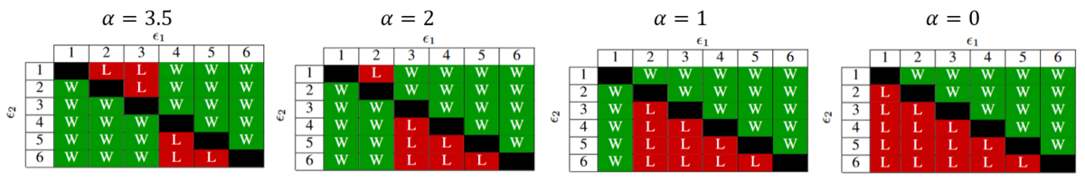Knowing about dice and probabilities, we can set $\alpha=3.5$ , which is the expected value of a fair dice. As seen in the leftmost table in Fig 1, from the 30 possible scenarios you will win in 24 in them, so we win more than half the time. You might say that $\alpha=3.5$ is a smart strategy since that is the expected value of a dice.

What if we pick something not so smart as our threshold? Setting $\alpha=2$ (cf., second table from left to right on Fig. 1) lowers the times we win to 23 out of 30 and setting $\alpha=1$ (cf., third table from left to right on Fig. 1) drops us down to 20 out of 30, which has us winning more than half the time in either scenario. The worst we can do is by setting $\alpha \geq 6$ or $\alpha\lt1$ where we win in only 15 of the 30 scenarios. Note that $\alpha\lt1$ is equivalent to never switching envelopes and $\alpha\gt6$ is equivalent to always switching envelopes and. Never switching envelopes and always switching envelopes is, basically, the same strategy (i.e., we randomly pick one envelope and stick to it) so we would win only half the time (cf., fourth table from left to right on Fig. 1).

Now you have proof of three things to be true in this simpler (call it “scaffolded”) version of our problem. First, we can win this game more than half the time. Second, if our value of $\alpha$ (i.e., what we consider “big enough”) is within the range of values we will see in the envelopes then we will win more than half the time. Third, knowing that ties are not possible (from the problem formulation we are told $\epsilon_1 \neq \epsilon_2$ ) is quite helpful information (i.e., the six events of equal values of the die are not possible outcomes).

For the curious: With a few lines of code you can computationally show that randomly picking $\alpha \in \{1,2,3,4,5,6\}$ in each round leads to winning more than half the time. Alternatively, you can work out the probabilities for each possible outcome of the dice and prove this mathematically which may be a fun exercise.

More abstractly

Now that we have evidence that we can win more than half the time, under some conditions, let’s take down some scaffolds and take a step into abstraction. Let us focus on our threshold, $\alpha$ , and consider three possible scenarios for the envelope values. The first scenario is when $\alpha$ is less than both envelope values (i.e., $\alpha \lt \epsilon_1$ and $\alpha \lt \epsilon_2$ ), the second scenario is when $\alpha$ is greater than both envelope values (i.e., $\alpha\gt\epsilon_1$ and $\alpha \gt \epsilon_2$ ), and the third scenario is when $\alpha$ is between both envelope values (i.e., $\epsilon_1 \lt \alpha \lt \epsilon_2$ or $\epsilon_2 \lt \alpha \lt \epsilon_1$ ). Note that the first and second scenarios can be subdivided depending on the relationship between $\epsilon_1$ and $\epsilon_2$ but, as you will see, this relationship is not required for our analysis.

When we are in the first scenario, we always keep the first envelope we open. When we are in the second scenario, we always switch our envelope. In both of these scenarios, assuming we randomly pick which envelope to look at first, we will (on average) win half of the times we play. For the third scenario, if we are in the case when $\epsilon_1 \lt \alpha \lt \epsilon_2$ we always switch envelopes and always win and if we are in the case when $\epsilon_2 \lt \alpha \lt \epsilon_1$ we always keep our envelope and win. Let that sink in for a moment.

To review, in the first and second scenario we will win half the time and in the third scenario we win all the time. The probability of winning among all scenarios is the weighted probability of each scenario (i.e., how often we win in a scenario multiplied by how often the scenario occurs). Therefore, we will win more than half the time as long as the third scenario occurs. Furthermore, our probability of winning directly depends on how often scenario 3 occurs.

For example, if all three scenarios are equally likely (i.e., scenario 1, scenario 2, and scenario 3 each occur one third of the time) then we, on average, win $\approx$ 66% of the times we play (i.e., 1/3 * 1/2 + 1/3 * 1/2 + 1/3 * 1= 2/3). As another example, if scenario 3 never occurs then we win 50% of the times we play (i.e., 1/2 * 1/2 + 1/2 * 1/2 + 0 * 1 = 1/2). As a final example, if scenario 3 happens half of the time and scenario 1 and 2 each happen 1/4 of the time then we win 75% of the times we play (i.e., 1/4 * 1/2 + 1/4 * 1/2 + 2/4 * 1 = 3/4).

Thinking about our results

From the approaches above we have learned that we can win more than half the time if our threshold is within the range of values we will see. How do we find a value within the range of values we will see? We could, very simply, use the first envelope value we see in our first game as our threshold. From the dice example, we can intuit that a smart approach is to guess the median value of whatever randomness is used to generate the numbers going into the envelopes. So maybe a smarter approach, assuming we have many games to play, is if we play a few games and update our estimate of the median as we go.

To get philosophical, we have (in a way) shown that it pays to be consistent even when faced with an unknown randomness (i.e., fixing $\alpha$ and winning more than half the time). To bring it back to my day-to-day work, the cellular network operated by DOCOMO must be given operating parameters (e.g., power levels and link assignments) even when each day we face a lot of unknown randomness (e.g., where users are, how users move, or the ambient temperature are all sources of randomness that impact the network). The smarter we are about picking parameters, then the better our network can operate.

Birthdays

The problem I describe below is popular among computer scientists as it relates to hash collisions or the “birthday attack”. Less known, perhaps, is how it relates to the surprisingly simple way that some wireless networks work and the real reason I like talking about this problem.

The train comes to a stop and you move with a hurried step. You arrive to the new tea shop you’ve heard so many great things, but you do so at exactly the same time as I do. Assuming we are equally polite we take turns insisting that the other person go first. To figure out who goes first we decide to flip a coin to see who orders first. But, what if three people arrive at the same time? Perhaps a few more complicated coin flips. And if ten people arrive at the same time? Assuming, again, we are all equally polite, we might need a system for deciding who should go first, second, third, and so on.

One such system might be that we each randomly pick a number and line up based on the number that we picked. For example, if there are ten of us then maybe we each pick a number between 1 and 10. Then, whoever picked 1 goes first, whoever picked 2 goes second, and so on. For clarity in exposition, we refer to the process of picking numbers and ordering as a “round”. To disincentivize people from always picking 1, whenever two (or more) people pick the same number they are made to wait and participate in the next round. For example, if two people pick 1 and the other eight people pick distinct numbers; the two people who picked 1 would wait for the other eight people to go in the first round then participate in a second round.

This system of randomly picking numbers will work, but not without hiccups. For example, if there are ten of us and we are picking numbers between 1 and 10 then it is very likely that many people will pick the same number and made to wait for subsequent rounds. Alternatively, if ten people randomly pick numbers between 1 and 1,000,000 then it is very unlikely that any two will pick the same number, but we will spend a long time sequentially asking for each number (e.g., "Did someone pick 90210? Did someone pick 90211?") to figure out who goes next*2. A small range of numbers leads to higher probability of people picking the same number but a larger range leads to longer rounds.

Given a number $P$ of people present, how big a range (call it $R$ ) should we pick? Furthermore, what is the probability that everyone goes this round (i.e., no two, or more, people pick the same number)?

Scaffolding to Some Understanding

If you know the birthday problem and feel comfortable with it, feel free to skip to the next part of this post. The most scaffolding we can do for this problem, without getting trivial, is to assume at least two people are present and our range is greater than one, i.e., $P\geq2$ and $R\gt1$ . Additionally, assume people will pick numbers in the range with uniform randomness (i.e., all numbers are equally likely to be picked). When thinking about the probability of you going this round, we are looking for events when every other number picked is different than yours. When thinking about the probability of everyone going this round, we are looking for events when all the numbers picked are distinct. If the difference is subtle, lets work out some simple examples. We focus on the latter type of thinking.

Start with just you and me (i.e., $P=2$ ), noting that any time that you get to go this round then everyone gets to go. With a range of 2, there are four possible events (i.e., we both pick 1, we both pick 2, you pick 1 and I pick 2, or you pick 2 and I pick 1) which are equally likely. Among these four possible events, in half of them we both get to go this round. With a range of 3 we have nine possible events from which only in three we do not go this round (i.e., we both pick the same number, be it 1, 2, or 3). Thus, in six of the nine events we both get to go this round. In general, when $P=2$ the probability of us picking the same number is $1/R$ and the probability of both of us picking different numbers is $(R-1)/R$ .

Things get interesting when we think of three people (i.e., $P=3$ ). First, note that if $R=2$ then the probability of you going this round is 1/4 (i.e., you pick a number and the other two people pick the other number) but the probability of all three people going in one round is 0 (i.e., two people, at least, pick the same number). For $R=3$ , the probability of everyone going this round is equal to 6/27 (i.e., from the possible 27 combinations in only six does everyone pick a different number). With $R=4$ , the the probability of everyone going this round is equal to 24/64. How do we know? Note, when we look for the events where everyone picks different numbers we are looking for all the combinations of picking $P$ numbers from $R$ without repeating and where order matters which is equal to $R!/(R-P)!$ (where $n!=n*(n-1)*(n-2)*...2*1$ ). When we look for all the possible events we are looking for all the possible combinations of picking one from $R$ numbers $P$ times which is equal to $R^{P}$ .

The probability of everyone going in one round is equal to

$\displaystyle P(\text{all go}) = \frac{\frac{R!}{(R-P)!}}{R^P} = \frac{R!}{R^P (R-P)!}$

\noindent while the probability of not everyone going in one round (i.e., at least two people pick the same number) is the complement, i.e.,

$\displaystyle P(\text{not all go}) = 1 - P(\text{all go}).$

Recall, for $P=3$ and $R=3$ we get $P(\text{all go})=6/27\approx 0.22$ , at $P=3$ and $R=4$ we get $P(\text{all go})=24/64 = 0.375$ , at $P=3$ and $R=5$ we get $P(\text{all go})=60/125\approx 0.48$ , and at $P=3$ and $R=6$ we get $P(\text{all go})=120/216\approx 0.55$ . Note, the probability of all going in one round keeps going up with a larger $R$ , but how much the probability increases with an increasing $R$ starts decreasing as $R$ grows. We must somehow decide how large a probability we are comfortable with. As a rule of thumb, when $N\approx \sqrt{R}$ we have $P(\text{all go}) \approx 0.5=P(\text{not all go})$ , meaning if we want about even odds for all people to go in one round we need the range to be at least equal to the square of the number of people wanting to go.

The fun part of the equation for $P(\text{all go})$ is how easily we can be deceived by factorial and exponential growth. The popular example of this deception is when we point out that for $R=365$ and $P=23$ then $P(\text{all go}) \approx 0.49$ which is often stated as “in a room with twenty-three people, it is more than likely than at least two people share the same birthday" and is often referred to as “the birthday problem". The deception comes in two ways. First, the statement is for the probability of any two people (or more) sharing the same birthday which is a very different statement than to say out of twenty-two people one will share your birthday.

The second deception, is in exponential (i.e., $R^{P}$ ) versus factorial growth (i.e., $R!$ ). Simplify the problem to consider finding when any two people from $N$ people pick the same random number out of a range $R$ . Notice there are $N*(N-1)/2$ comparisons we need to make among $N$ people when trying to find if any two picked the same number, e.g., if $N=2$ we need to make 1 comparison, if $N=3$ we need to make 3 comparisons, if $N=4$ we need to make 6 comparisons, and for $N=23$ we need to make 253 comparisons. Rethink making a comparison as flipping an unfair coin. The unfair coin, let say, shows heads tex: 99.7% of the time and tails only 0.3% of the time. You expect the unfair coin to show heads when you flip it once. You expect the unfair coin to show ten heads in a row when you flip it ten times. Do you expect to see 253 heads in a row when you flip the unfair coin 253 times? The number of coin flips we need to do grows quickly with $N$ while increasing $R$ will, in this analogy, increase the probability of our unfair coin landing in heads but never gets to 100%.

David, do you organize people in line for tea or do you work with wireless networks?

How does the famous “birthday problem" relate to wireless networks? One way users communicate on a wireless network is through random access. In random access, users will “randomly” start talking but we want to avoid more than one user talking at the same time. Thinking back to our analogy, your wireless devices are the people getting in line and putting in tea orders would be equivalent to communicating across the network. The benefit of random access is that it is totally decentralized and requires minimal overhead to setup, this allows users to come in and out of the network seamlessly.

In random access, users pick a random number from predetermined range and begin counting down from that number until reaching zero to then transmit. If another user picked the same number we have what is called a “collision". In the tea order analogy before we could see how many people there are and could coordinate to decide a range. One aim of random access is to minimize coordination, meaning users are not made aware of how many other users there are or not in the network. Thus, upon collision a user will increase the range from which they randomly pick a number, i.e., a collision implies the range was not large enough, so we make it bigger for the next round. Alternatively, no collision suggests that the range might be too large for the number of users.

Putting things together

In the envelope problem, having a second opportunity at a random number, i.e. switching our envelope, let us win more than half the times. That extra chance, even with an unknown randomness, allowed us to do better than what intuition might originally suggest.

In the birthday problem, every other person represents not just one opportunity for a collision but a new opportunity for a collision for each person already accounted for. Thus, what seems like an unlikely event (i.e., a collision) becomes expected to happen given the quickly growing number of opportunities. Collisions happen quite often over wireless networks, and they are part of the cost we pay to provide mobility to users.

I hope you’ve enjoyed learning about a couple of fun math problems with randomness. Additionally, I hope you have seen the power of scaffolding when approaching “hard” problems which was my secret goal from this blog post. If you want to know more about “scaffolding" or how to approach hard looking problems, I strongly recommend George Polya’s book titled “How to Solve It" a wonderful book accessible to everyone regardless of mathematical skill level.

A big part of my day-to-day work is dealing with randomness and helping pick numbers within all this randomness. If you want to learn more about the math, topics such as probability, statistics, optimization (e.g., combinatorial optimization and stochastic optimization), and information theory might be of interest to you. For the engineering aspect, topics on computer networks and communication theory might be of interest to you.

Author: David Ramirez

*1:Mt. Komaki is listed as the smallest hill in Japan in Wikipedia’s article “List of mountains and hills in Japan by height”.

*2:There are quicker ways of figuring out who goes next where we do not sequentially ask for every number, but for this post lets only consider methods with round duration that grows with the range of numbers.