Day 15 of NTT DOCOMO R&D Advent Calendar 2022

One Equals One

In my role as a Senior Research Engineer at DOCOMO Innovations I get to help optimize how our mobile communication network operates. This often means wrangling a lot of complex math and wrapping my head around many moving pieces of the network. A network is a complex system made up of many interconnected systems. There is much to learn about the complex by understanding the simple. To remind us of this, let us remember a fun fact that maybe has not crossed your mind in a while:

$\displaystyle 1 = 1 + (1 - 1).$

In what follows, I will take this simple fun fact and show how it is part of several mathematical results and present in a communication network.

The One and the Missing Tea

First, let’s retell a story often told as three people inheriting seventeen camels. This retelling goes as follows: Seventeen boba teas are delivered to the office and the intent is to distribute these to three departments in proportion to their size of the entire office. Department A counts for half the office so they should receive half the teas, Department B is a third of the office and should receive one third of the teas, and Department C is one ninth of the office and should receive one ninth of the teas. With $17$ teas, Department A would get $8.5$ teas, Department B would get $5 \frac{2}{3}$ teas, and Department C would get $1 \frac{8}{9}$ teas.

Nobody in Department A is interested in half a boba tea, or less, especially when considering whoever gets “the first half” gets all the tapioca! Before things escalate into a tea dispute, HR is called and they send someone who read this post. The HR employee offers their own tea, thus bringing the count of total teas to 18. Department A takes 9 teas, Department B takes 6 teas, and Department C takes 2 teas. Note that $9+6+2=17$ so the HR employee can take their tea back.

All the HR employee had to to solve this conflict was to add one then subtract one. Equality was never broken (we split the same total number of teas before and after HR showed up), but what did happen was that the computations became easier (we were able to split the teas without sharing an individual tea). Basically, $17 = 17 + (1 - 1)$ .

The One and the Quadratic Equation

Here is a more abstract version of what we are talking about

$\displaystyle x = x+(y-y).$

Let’s go beyond splitting teas to the quintessential math problem of solving for $x$ when $a,b,c$ are constants in

$\displaystyle a x^2 + bx + c = 0.$

If you thought “Oh, easy, I’ll use the quadratic equation”, i.e.,

$\displaystyle x = \frac{-b \pm \sqrt{b^2 - 4ac}}{2a},$

then you’re thinking about using a result derived using the fact that $x = x+(y-y)$ . How? First, we factor $a$ from the equation $ax^{2} + bx + c = 0$ . Second, via the fact that $x=x+(y-y)$ , we add and subtract the value of $\frac{b^{2}}{4a^{2}}$ . In math, this looks as

$\displaystyle \begin{split} a x^2 + bx + c & = a \left[ x^2 + \frac{b}{a}x + \frac{c}{a} \right] \\ & = a \left[ x^2 +\frac{b}{a} x + \frac{b^2}{4a^2} - \frac{b^2}{4a^2} + \frac{c}{a} \right] \\ & = a \left[ \left( x + \frac{b}{2a} \right)^2 - \frac{b^2}{4a^2} + \frac{c}{a} \right] = 0 \end{split}$

Next, we rearrange and clear the value of $x$ on one side

$\displaystyle \begin{split} \left( x+ \frac{b}{2a} \right) ^2 & = \frac{b^2 - 4ac}{4a^2} \\ x + \frac{b}{2a} & = \frac{\pm \sqrt{b^2-4ac}}{2a} \\ x & = \frac{-b \pm \sqrt{b^2-4ac}}{2a} \end{split}$

The One and a Function of a Function

Let’s move up from adding and subtracting the same element into multiplying and dividing by the same element, i.e.,

$\displaystyle x = x * \frac{y}{y}.$

Instead of quadratic equations let’s think about derivatives of composite functions. A composite function is a function that uses as input the output of another function. Basically, a composite function is a function of a function. A derivative of a composite function is obtained by solving

$\displaystyle \begin{split} (f \circ g)'(x) & = \lim_{\epsilon \rightarrow 0} \frac{f(g(x)) - f(g(\epsilon))}{x-\epsilon} \end{split}$

We can solve this from the fact that $x = x* \frac{y}{y}$ . We multiply and divide by $g(x)-g(\epsilon)$ and then group into terms we recognize. In math, this is as follows

$\displaystyle \begin{split} (f \circ g)'(x) & = \lim_{\epsilon \rightarrow 0} \frac{f(g(x)) - f(g(\epsilon))}{x-\epsilon} \frac{g(x)-g(\epsilon)}{g(x)-g(\epsilon)} \\ & = \lim_{\epsilon \rightarrow 0} \frac{f(g(x)) - f(g(\epsilon))}{g(x)-g(\epsilon)} \frac{g(x)-g(\epsilon)}{x-\epsilon} \\ & = \lim_{\epsilon \rightarrow 0} \frac{f(g(x)) - f(g(\epsilon))}{g(x)-g(\epsilon)} \lim_{\epsilon \rightarrow 0} \frac{g(x)-g(\epsilon)}{x-\epsilon} \\ & = f'(g(x)) \cdot g'(x) \end{split}$

and thus we get what is often called the chain rule *1. The chain rule gets used in backpropagation which is a training algorithm for neural networks, gradient descent for finding optimal operating points, and more!

The Noisy One

So far we’ve introduced and removed a carefully selected value. Can we get a good result from adding some random value? Short answer: yes! Dithering is when we intentionally add a random value into our equation and can be quite helpful. We will first introduce the concepts, use an analogy to gain some understanding, then highlight some results obtained via dithering.

We use dithering when quantization is involved. Quantization occurs when converting an analog signal (e.g., your voice) into a digital signal (e.g., a voice note on your phone). Anytime you make a call on your mobile phone, your voice is quantized before it is heard by the receiver. Broadly speaking, quantization is when we take a thing that can be one of many values and convert it into a similar thing that can be one of fewer values. Taking any number between $1$ and $10$ and quantizing it to an even number between $1$ and $10$ can result in quantization error no greater than $1$ (e.g., quantizing $1$ into $2$ gives us an error of $1$ ). Next, let’s go through an analogy to explain these concepts.

Your favorite tea shop suddenly changes their menu and offers only half of their original items, we could say they quantized the menu. Your favorite tea is no longer on the menu, but there’s a few teas on there with a similar flavor profile. The difference between your favorite tea and the tea you end up getting would be the quantization noise.

For exposition, know that there is subtractive dithering (when the random value is added and subtracted) and non-subtractive dithering (when the random value is added but not subtracted). In theory, subtractive dithering is quite helpful. In practice, non-subtractive dithering is easier to apply due to system limitations.

For example, one can show that if using subtractive dithering then quantization noise is statistically independent for any input. For comparison, adding noise depending on the input is part of how noise cancelling headphones work (i.e., add “noise” that is the inverse of the input from outside the headphones). Recalling our analogy with the tea shop reducing the menu, if we go to the tea shop many times and randomly pick one of the few teas closest in flavor to our favorite tea, then we can perceive as if we are still enjoying our favorite tea even when no one individual tea is our favorite! The random picking of a similar tea flavor is dithering and that perceived effect of retaining the original flavor of our favorite tea is why we do dithering. When your voice is quantized an error is introduced, but with dithering we can achieve the perception that the voice went by apparently (i.e., on the average) without error from the receiver’s perspective.

In practice, we cannot subtract the dithering effect from our tea selection. Also in practice, subtractive dithering is hard to implement other than for very simple cases*2. Instead of going into higher level math, which is nicely detailed in here or a more recent take here. Instead, we will see the power of dithering by focusing on non-subtractive dithering.

Figure 1. Left to right: Color image, black and white image with arbitrary quantization, black and white image with Floyd–Steinberg dithering, black and white image with ordered dithering.

Figure 2. Left to right: Closeup of bird portrait in color image, black and white image with arbitrary quantization, black and white image with Floyd–Steinberg dithering, and black and white image with Ordered dithering.

The One Visual Example

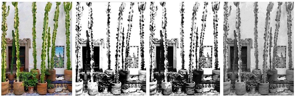
Recall, non-subtractive dithering is randomly adding an element and we use it when quantizing. Consider the images shown in Fig. 1. The left-most image is a color image of some pretty tall plants somewhere in Mexico. We can “quantize” the colors in this image into either black and white. The second image from left to right quantizes simply by looking at the intensity of the colors in the original image and deciding arbitrarily to turn a pixel into either black or white. A lot of the image quality is lost (e.g., the sky in the bird painting becomes simply white). The third image from left to right does what is called Floyd-Steinberg dithering where noise is introduced to the quantization decision in the form of a sliding window of the error caused by previous decisions (e.g., some of the sky in the bird painting survives quantization). Basically, the noise comes from the image itself where if a series of pixels was making you decide for one color it becomes more likely (but not guaranteed) that you’ll decide for the other color in the next pixel. The fourth (and right most) image does quantization with Ordered dithering where noise is applied in an arbitrary pattern repeated throughout the entire image. You can make out the crosshatch pattern in many parts of the image since each point in the pattern has a different noise value. This repeated pattern is adding a fixed noise to whichever pixel it so happens to land at, each pixel having a distinct noise value added. In fact, one such value is $0$ and happens at the top-left corner of our pattern, if you look carefully in the image you will notice this repeating white valued pixel that helps discern the pattern.

To better appreciate the differences from dithering, Fig. 2 has a close up of the bird portrait (right side of the picture) following the same order as described in Fig. 1. Now, quantization is forcing us to lose some of the image. We go from a wide range of colors to simply black or white. Yet, by adding noise we can create images that become more visually appealing or better representations of the original image.

Concluding One

Thus, by including a value then removing that value we are able to obtain some useful results. Similarly, by simply adding a value in a careful manner we are able to produce more aesthetically pleasing results when quantizing. A lot of “knowing math” is simply knowing what tool to use. Knowing what tool to use becomes easier when we better understand the simplest of our tools.

Author: David Ramirez

*1:The ever astute reader will note there is one hidden step to handle division by zero.

*2:For the interested reader, learning about dynamic range of digital-to-analog converters can elucidate more of the technical challenges for practical use of subtractive dithering.